Neural Network Activation Functions With Tensorflow

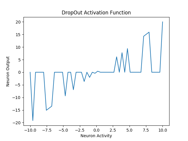
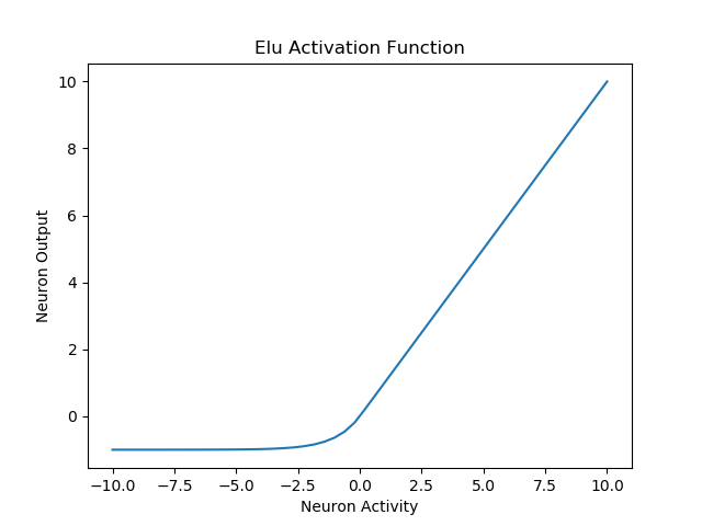
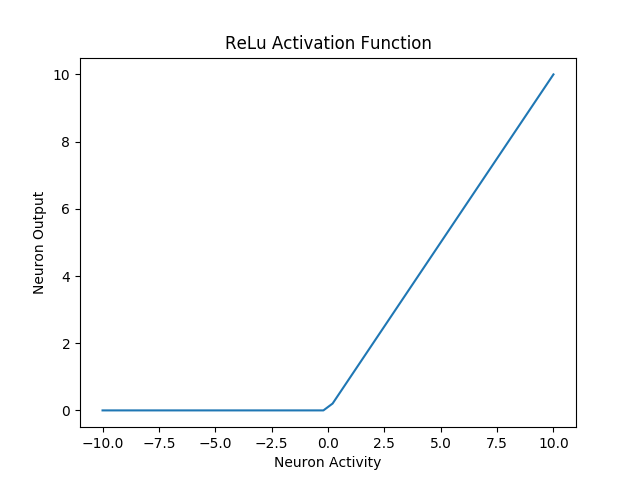
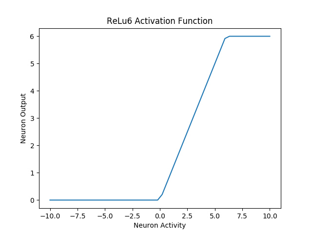
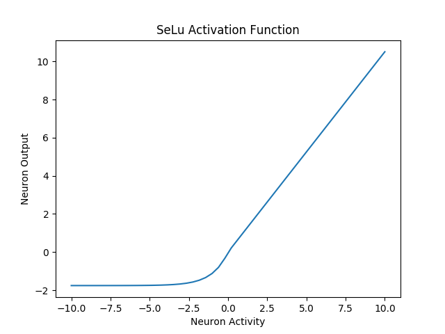
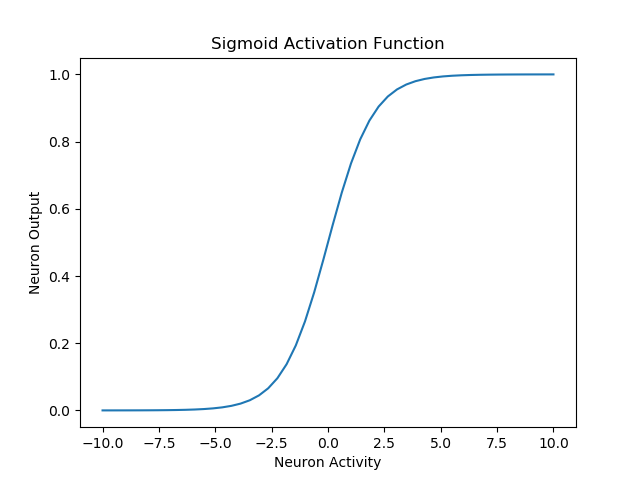
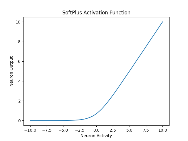
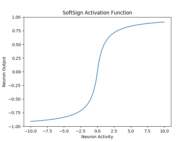
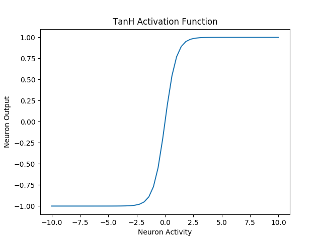
Neural network activation functions influence neural network behavior in that they determine the fire or non-fire of neurons. ReLu is the one that is most commonly used currently. The visualizations below will help us to understand them more intuitively and there are code samples so that you can run it on your machine.

Dropout

1
2
3
4
5
6
7
8
9
10
11
12
13
14
15
16
17
#Tensorflow 1.x
import tensorflow as tf
import numpy as np
import matplotlib.pyplot as plot

x = np.linspace(-10, 10, 50)
output = tf.nn.dropout(x, 0.5)
initialization = tf.global_variables_initializer()

with tf.Session() as session:
session.run(initialization)
y = session.run(output)
plot.xlabel('Neuron Activity')
plot.ylabel('Neuron Output')
plot.title('DropOut Activation Function')
plot.plot(x, y)
plot.show()

Figure 1 : DropOut Activation Function

Elu

1
2
3
4
5
6
7
8
9
10
11
12
13
14
15
16
17
18
19
20
21
22
23
24
25
26
27
28
29
30
#Tensorflow 1.x
import tensorflow as tf
import numpy as np
import matplotlib.pyplot as plot

x = np.linspace(-10, 10, 50)
output = tf.nn.elu(x)
initialization = tf.global_variables_initializer()

with tf.Session() as session:
session.run(initialization)
y = session.run(output)
plot.xlabel('Neuron Activity')
plot.ylabel('Neuron Output')
plot.title('Elu Activation Function')
plot.plot(x, y)
plot.show()

#Tensorflow 2.x
import tensorflow as tf
import numpy as np
import matplotlib.pyplot as plot

x = np.linspace(-10, 10, 50)
y = tf.keras.activations.elu(x)
plot.xlabel('Neuron Activity')
plot.ylabel('Neuron Output')
plot.title('Elu Activation Function')
plot.plot(x, y)
plot.show()

Figure 2 : Elu Activation Function

ReLu

1
2
3
4
5
6
7
8
9
10
11
12
13
14
15
16
17
18
19
20
21
22
23
24
25
26
27
28
29
30
#Tensorflow 1.x
import tensorflow as tf
import numpy as np
import matplotlib.pyplot as plot

x = np.linspace(-10, 10, 50)
output = tf.nn.relu(x)
initialization = tf.global_variables_initializer()

with tf.Session() as session:
session.run(initialization)
y = session.run(output)
plot.xlabel('Neuron Activity')
plot.ylabel('Neuron Output')
plot.title('ReLu Activation Function')
plot.plot(x, y)
plot.show()

#Tensorflow 2.x
import tensorflow as tf
import numpy as np
import matplotlib.pyplot as plot

x = np.linspace(-10, 10, 50)
y = tf.keras.activations.relu(x)
plot.xlabel('Neuron Activity')
plot.ylabel('Neuron Output')
plot.title('Relu Activation Function')
plot.plot(x, y)
plot.show()

Figure 3 : ReLu-Activation-Function

ReLu6

1
2
3
4
5
6
7
8
9
10
11
12
13
14
15
16
17
#Tensorflow 1.x
import tensorflow as tf
import numpy as np
import matplotlib.pyplot as plot

x = np.linspace(-10, 10, 50)
output = tf.nn.relu6(x)
initialization = tf.global_variables_initializer()

with tf.Session() as session:
session.run(initialization)
y = session.run(output)
plot.xlabel('Neuron Activity')
plot.ylabel('Neuron Output')
plot.title('ReLu6 Activation Function')
plot.plot(x, y)
plot.show()

Figure 4 : ReLu6-Activation-Function

SeLu

1
2
3
4
5
6
7
8
9
10
11
12
13
14
15
16
17
18
19
20
21
22
23
24
25
26
27
28
29
30
31
#Tensorflow 1.x
import tensorflow as tf
import numpy as np
import matplotlib.pyplot as plot

x = np.linspace(-10, 10, 50)
output = tf.nn.selu(x)
initialization = tf.global_variables_initializer()

with tf.Session() as session:
session.run(initialization)
y = session.run(output)
plot.xlabel('Neuron Activity')
plot.ylabel('Neuron Output')
plot.title('SeLu Activation Function')
plot.plot(x, y)
plot.show()

#Tensorflow 2.x
import tensorflow as tf
import numpy as np
import matplotlib.pyplot as plot

x = np.linspace(-10, 10, 50)
y = tf.keras.activations.selu(x)
plot.xlabel('Neuron Activity')
plot.ylabel('Neuron Output')
plot.title('Selu Activation Function')
plot.plot(x, y)
plot.show()

Figure 5 : SeLu Activation Function

Sigmoid

1
2
3
4
5
6
7
8
9
10
11
12
13
14
15
16
17
18
19
20
21
22
23
24
25
26
27
28
29
30
#Tensorflow 1.x
import tensorflow as tf
import numpy as np
import matplotlib.pyplot as plot

x = np.linspace(-10, 10, 50)
output = tf.nn.sigmoid(x)
initialization = tf.global_variables_initializer()

with tf.Session() as session:
session.run(initialization)
y = session.run(output)
plot.xlabel('Neuron Activity')
plot.ylabel('Neuron Output')
plot.title('Sigmoid Activation Function')
plot.plot(x, y)
plot.show()

#Tensorflow 2.x
import tensorflow as tf
import numpy as np
import matplotlib.pyplot as plot

x = np.linspace(-10, 10, 50)
y = tf.keras.activations.sigmoid(x)
plot.xlabel('Neuron Activity')
plot.ylabel('Neuron Output')
plot.title('Sigmoid Activation Function')
plot.plot(x, y)
plot.show()

Figure 6 : Sigmoid Activation Function

SoftPlus

1
2
3
4
5
6
7
8
9
10
11
12
13
14
15
16
17
18
19
20
21
22
23
24
25
26
27
28
29
30
#Tensorflow 1.x
import tensorflow as tf
import numpy as np
import matplotlib.pyplot as plot

x = np.linspace(-10, 10, 50)
output = tf.nn.softplus(x)
initialization = tf.global_variables_initializer()

with tf.Session() as session:
session.run(initialization)
y = session.run(output)
plot.xlabel('Neuron Activity')
plot.ylabel('Neuron Output')
plot.title('SoftPlus Activation Function')
plot.plot(x, y)
plot.show()

#Tensorflow 2.x
import tensorflow as tf
import numpy as np
import matplotlib.pyplot as plot

x = np.linspace(-10, 10, 50)
y = tf.keras.activations.softplus(x)
plot.xlabel('Neuron Activity')
plot.ylabel('Neuron Output')
plot.title('SoftPlus Activation Function')
plot.plot(x, y)
plot.show()

Figure 7 : SoftPlus-Activation-Function

SoftSign

1
2
3
4
5
6
7
8
9
10
11
12
13
14
15
16
17
18
19
20
21
22
23
24
25
26
27
28
29
30
#Tensorflow 1.x
import tensorflow as tf
import numpy as np
import matplotlib.pyplot as plot

x = np.linspace(-10, 10, 50)
output = tf.nn.softsign(x)
initialization = tf.global_variables_initializer()

with tf.Session() as session:
session.run(initialization)
y = session.run(output)
plot.xlabel('Neuron Activity')
plot.ylabel('Neuron Output')
plot.title('SoftSign Activation Function')
plot.plot(x, y)
plot.show()

#Tensorflow 2.x
import tensorflow as tf
import numpy as np
import matplotlib.pyplot as plot

x = np.linspace(-10, 10, 50)
y = tf.keras.activations.softsign(x)
plot.xlabel('Neuron Activity')
plot.ylabel('Neuron Output')
plot.title('SoftSign Activation Function')
plot.plot(x, y)
plot.show()

Figure 8 : SoftSign Activation Function

TanH

1
2
3
4
5
6
7
8
9
10
11
12
13
14
15
16
17
18
19
20
21
22
23
24
25
26
27
28
29
30
31
#Tensorflow 1.x
import tensorflow as tf
import numpy as np
import matplotlib.pyplot as plot

x = np.linspace(-10, 10, 50)
output = tf.nn.tanh(x)
initialization = tf.global_variables_initializer()

with tf.Session() as session:
session.run(initialization)
y = session.run(output)
plot.xlabel('Neuron Activity')
plot.ylabel('Neuron Output')
plot.title('TanH Activation Function')
plot.plot(x, y)
plot.show()

#Tensorflow 2.x
import tensorflow as tf
import numpy as np
import matplotlib.pyplot as plot

x = np.linspace(-10, 10, 50)
y = tf.keras.activations.tanh(x)
plot.xlabel('Neuron Activity')
plot.ylabel('Neuron Output')
plot.title('TanH Activation Function')
plot.plot(x, y)
plot.show()

Figure 9 : TanH Activation Function

Time series market prediction using neural networks

Tensorflow is used to predict future price values on the time series financial market.

Input data

Input data is acquired via the MT5 terminal.

Imports

1
2
3
4
5
6
7
8
9
10
11
12
13
14
15
16
17
18
19
20
from __future__ import absolute_import, division, print_function, unicode_literals
import warnings
warnings.filterwarnings("ignore")
import pathlib
import matplotlib.pyplot as plt
import pandas as pd
import seaborn as sns
import tensorflow as tf
from tensorflow import keras
from tensorflow.keras import layers
print("Tensorflow Version : " + tf.__version__)
import sys
print("Python Version : " + sys.version)
from tensorflow.python.client import device_lib
print(device_lib.list_local_devices())
from sklearn import preprocessing
import numpy as np
from numpy.random import seed
import winsound
import os

AI Model Save

These variables allow for the AI model to be saved.

1
2
checkpoint_path = "C:\\Users\\41507\\AppData\\Roaming\\MetaQuotes\\Terminal\\158904DFD898D640E9B813D10F9EB397\\MQL5\\Files\\ModelClose\\EURUSD\\modelClose.ckpt"
checkpoint_dir = os.path.dirname(checkpoint_path)

Data Import

Import the data from csv.

1
df = pd.read_csv('C:\\Users\\41507\\AppData\\Roaming\\MetaQuotes\\Terminal\\158904DFD898D640E9B813D10F9EB397\\MQL5\\Files\\EUR_USD_Test_H1.csv', header=0, delimiter=r"\s+")

Data Shape

Look at the shape of the data.

1
print(df.shape)

Clean Data

Clean the data and create columns for looking back.

1
2
3
4
5
6
7
8
9
10
11
12
13
14
15
16
17
18
19
20
21
22
23
24
25
26
27
28
29
30
31
32
33
34
35
36
37
38
39
40
41
42
43
44
45
46
47
48
49
50
51
52
53
54
55
56
57
58
59
60
df.columns = df.columns.str.replace("<", "")
df.columns = df.columns.str.replace(">", "")
# Extract date features
df['DATE'] = df['DATE'].astype('datetime64[ns]')
df['day_of_year'] = df['DATE'].dt.dayofyear
df['year'] = df['DATE'].dt.year

#Save Date in another dataframe for later use and then delete
dfDate = pd.DataFrame(df, columns=['DATE', 'TIME'])
del df['DATE']

df['TIME'] = df['TIME'].astype('datetime64[ns]')
df['hour_of_day'] = df['TIME'].dt.hour

#Save Time in another dataframe for later use and then delete
dfTime = pd.DataFrame(df, columns=['TIME'])
del df['TIME']

# Add column minmaxdiff
#df['score_diff'] = df['HIGH'].sub(df['LOW'], axis = 0)
#df['min_max_next'] = (df['HIGH']+df['LOW'])/2

# Add columns for previous candles
df['OPEN1'] = df['OPEN'].shift(1)
df['HIGH1'] = df['HIGH'].shift(1)
df['LOW1'] = df['LOW'].shift(1)
df['CLOSE1'] = df['CLOSE'].shift(1)
df['OPEN2'] = df['OPEN'].shift(2)
df['HIGH2'] = df['HIGH'].shift(2)
df['LOW2'] = df['LOW'].shift(2)
df['CLOSE2'] = df['CLOSE'].shift(2)
df['OPEN3'] = df['OPEN'].shift(3)
df['HIGH3'] = df['HIGH'].shift(3)
df['LOW3'] = df['LOW'].shift(3)
df['CLOSE3'] = df['CLOSE'].shift(3)
df['OPEN4'] = df['OPEN'].shift(4)
df['HIGH4'] = df['HIGH'].shift(4)
df['LOW4'] = df['LOW'].shift(4)
df['CLOSE4'] = df['CLOSE'].shift(4)
df['OPEN5'] = df['OPEN'].shift(5)
df['HIGH5'] = df['HIGH'].shift(5)
df['LOW5'] = df['LOW'].shift(5)
df['CLOSE5'] = df['CLOSE'].shift(6)
df['OPEN6'] = df['OPEN'].shift(6)
df['HIGH6'] = df['HIGH'].shift(6)
df['LOW6'] = df['LOW'].shift(6)
df['CLOSE6'] = df['CLOSE'].shift(6)
df['OPEN7'] = df['OPEN'].shift(7)
df['HIGH7'] = df['HIGH'].shift(7)
df['LOW7'] = df['LOW'].shift(7)
df['CLOSE7'] = df['CLOSE'].shift(7)
df['OPEN8'] = df['OPEN'].shift(8)
df['HIGH8'] = df['HIGH'].shift(8)
df['LOW8'] = df['LOW'].shift(8)
df['CLOSE8'] = df['CLOSE'].shift(8)
df['OPEN9'] = df['OPEN'].shift(9)
df['HIGH9'] = df['HIGH'].shift(9)
df['LOW9'] = df['LOW'].shift(9)
df['CLOSE9'] = df['CLOSE'].shift(9)
df.fillna(0, inplace=True)

Add Label

This is the value that will be predicted. The value is the close price of the next bar.

1
2
step = -1
df['prediction_output'] = df['CLOSE'].shift(step)

Split the data into train and test

80% of the data will be used for training and 20% will be used for testing.

1
2
3
4
n = 80
train_dataset = df.head(int(len(df)*(n/100)))
test_dataset = df.drop(train_dataset.index)
dfDate = dfDate.drop(train_dataset.index)

Split features from labels

1
2
3
4
5
train_labels = train_dataset.pop('prediction_output')
test_labels = test_dataset.pop('prediction_output')
# Compare the shapes
print(train_labels.shape)
print(test_labels.shape)

Normalize the data

1
2
3
4
5
6
def norm(x):
return (x - train_stats['mean']) / train_stats['std']
normed_train_data = norm(train_dataset)
del normed_train_data['prediction_output']
normed_test_data = norm(test_dataset)
del normed_test_data['prediction_output']

Build the model

The model has 5 layers and a learning rate of 0.003.

1
2
3
4
5
6
7
8
9
10
11
12
13
14
15
def build_model():
model = keras.Sequential([
layers.Dense(64, activation=tf.nn.relu, input_shape=[len(normed_train_data.keys())]),
layers.Dense(128, activation=tf.nn.relu),
layers.Dense(64, activation=tf.nn.relu),
layers.Dense(1)
])

optimizer = tf.keras.optimizers.RMSprop(learning_rate=0.003, rho=0.9)

model.compile(loss='mean_squared_error',
optimizer=optimizer,
metrics=['mean_absolute_error', 'mean_squared_error'])
return model

Train the model

The model training has 1000 epochs and a patience value of 100.

1
2
3
4
5
6
7
8
9
10
11
12
13
14
15
16
17
18
19
20
21
22
23
model = build_model()
model.summary()
# Display training progress by printing a single dot for each completed epoch
class PrintDot(keras.callbacks.Callback):
def on_epoch_end(self, epoch, logs):
if epoch % 100 == 0: print('')
print('.', end='')

EPOCHS = 1000

# The patience parameter is the amount of epochs to check for improvement
early_stop = keras.callbacks.EarlyStopping(monitor='val_loss', patience=100)

# Create a callback that saves the model's weights
cp_callback = tf.keras.callbacks.ModelCheckpoint(filepath=checkpoint_path,
save_weights_only=True,
verbose=0)

history = model.fit(normed_train_data, train_labels, epochs=EPOCHS,
validation_split = 0.2, verbose=0, callbacks=[early_stop, PrintDot(), cp_callback])
hist = pd.DataFrame(history.history)
hist['epoch'] = history.epoch
hist.tail()

Results

1
2
3
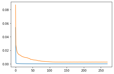
loss, mae, mse = model.evaluate(normed_test_data, test_labels, verbose=0)
print("Testing set Mean Abs Error: {:6.4f}".format(mae))
print("Testing set Mean Squared Error: {:6.4f}".format(mse))
1
2
Testing set Mean Abs Error: 0.0011
Testing set Mean Squared Error: 0.0002
1
2
3
4
# plot calculated metrics
plt.plot(history.history['mean_squared_error'])
plt.plot(history.history['mean_absolute_error'])
plt.show()

forex-prediction-results

The model can predict the closing price of the next bar with a MAE(mean absolute error) of 11 pips.
Cross validation will make the result more robust.